Implementation: overview

These pages document the implementation of the numerical experiments for paper “On Aligning Non-Order-Associated Binary Decision Diagrams” by Bochkarev and Smith. The notes along with the accompanying source code and data are assumed to provide enough information to:

1. inspect the raw data,

2. reproduce / adjust / inspect the figures from the paper (given the experiment log files) as necessary, and

3. completely reproduce the paper results from scratch, including instance generation.

It is our special interest to help the reader build upon our results, so please do not hesitate to address any technical questions to Alexey Bochkarev.

Computational infrastructure

To run the experiments we used machines running GNU/Linux system (remote computational resources provided by Clemson Palmetto cluster and laptops), running the following software:

• experiments implementation: python3. packages list, the usual way should work:

  pip install -r requirements.txt
  

• figures: R. To install (a superset of) the necessary libraries, from within R session:

install.packages(c("dplyr", "ggplot2", "ggridges",
   "gridExtra", "latex2exp", "optparse", "reshape",
   "stringr", "tidyr", "viridis", "xtable"))

• parallel computation: GNU parallel,

• experiments pipeline: GNU make and PBS (for job scheduling on the cluster).

• (we also used a separate tool to receive the results promptly via Telegram, but this can be safely removed)

• numerical experiments require Gurobi solver.

• most graphs were visualized used a stand-alone program called Graphviz Note that before pip install pygraphviz you might need to install the program and the header files as well. On my Debian distribution I needed to do sudo apt install graphviz graphviz-dev.

Note

For the (python) environment management we used the recommended venv-way. For example, the virtual environment can be created and activated with:

$ python3.10 -m venv .venv
$ source .venv/bin/activate

$ # then, we can install the necessary packages there with:

$ pip install -r requirements.txt

An equivalent for conda-based system would be:

$ conda create --name py310 python=3.10
$ conda install --name py310 --channel conda-forge --file requirements.txt
$ conda activate py310

(However, we did not use conda. If you do – please, let us know if it works as well.)

General reproducibility

Assuming the necessary software is present, one can rebuild any figure from the existing log file (specific experiment results) by running a make command from the root project directory (align-BDD). For example, this must work (assuming the necessary dependencies are installed):

make figures/simpl_heuristics.eps  # to rebuild Figure 6, or
make figures  # to rebuild all figures for the paper

GNU make will consider files’ timestamps and re-run the experiments as necessary (e.g., if the instance generation procedure has changed). To force a complete run (generate all the data, make all experiments, and build all figures), just clean up the previous results first:

make fresh  # to delete all instances and run logs
make figures  # to rebuild everything

Note, however, that depending on the parameters (which are set in Makefile) and the hardware, it might take quite some time to recalculate everything. PBS scripts that were used to run our experiments on the computation cluster are kept in folder 📁 pbs. Certainly, they are dependent on the hardware and the available software, but these materials hopefully will provide a good starting point to reproduce the results presented in the paper using a PBS-based system.

All the recipies (how to make each figure or other artifact) are described in the file called Makefile, which is basically a list of commands and source files needed to build each target.

Project repository structure.

All the source data is available in the project repository.

Key folders are:

• 📁 instances: all the instance (“raw”) data in a compressed format (tar.gz; see e.g. here if unsure how to open it),

• 📁 run_logs: all the numerical results – “run logs,” mostly as comma separated files (.csv)

• 📁 experiments and the root folder contain all key implementation files (in Python).

• 📁 post_processing: the R code that produces figures from the run logs.

• 📁 figures: the key figures themselves.

• 📁 docs: the code documentation source (i.e., these pages).

• 📁 tests: most of the code testing (for python code).

• 📁 pbs: auxiliary PBS scripts used to run the code on the computational cluster.

The computations are summarized in the following table (scrollable right):

Figure / Table	Filename	Experiments code (scripts)	Raw instances	Format	Experiment run log	Plotting code
Table 1	guessing.tex	gen_BDD_pair + solve_inst	orig_problem.tar.gz	BDD	main_rnd_run.csv	tab_guessing.R
Figure 6	simpl_heuristics.eps					fig_simpl_heuristics.R
Figure 7	orig_obj_histograms.eps					fig_obj_hist.R
Figure 17	LB.eps	gen_BDD_pair + experiments.compare_simpl_LBs			simpl_LB.csv	fig_LBs.R
Figure 19	orig_lwidth_stats.eps	gen_BDD_pair + experiments.gen_lsizes_stats	orig_stats.tar.gz		lwidths.csv	fig_summary.R
Figure 8	orig_runtimes.eps	gen_BDD_pair + experiments.par_scal_test	orig_scal.tar.gz		orig_scal.csv	fig_scal.R
Figure 20 Figure 21 Figure 22 Figure 23	no_opts.eps opts_diam.eps heuristic_simscore.eps heuristic_simscore_vs_AB_simscore. eps	gen_BDD_pair + experiments.heu_sol_struct	heu_sol_struct.tar.gz		simpl_sol_struct.csv	fig_simpl_opt_struct.R
Figure 9b Figure 10a Figure 10b	tMIP_tMIPCPP_tDD.eps intDD_VS_vs_toA.eps tMIP_tMIPCPP_tDD.eps	UFLP_2_cav darkcloud.gen_caveman_inst() jUFLP_cavemen jUFLP_utils experiments.softcover.generate_overlaps()	jUFLP.tar.gz	json	2022-07-19_jUFLP.csv	fig_DDvsMIP.R
Figure 11	fig_jUFLP_simscores.eps	experiments.jUFLP_w_simscores	jUFLP_ss.tar.gz	json	2022-12-06_jUFLP_simscores.csv	jUFLP_simscores.R

Figure 17: sample branch and bound tree was generated by experiments.sample_BB_tree.

Figures 1-5, 9a, 12-16, and 24-27 do not involve any computations.

Key ‘global’ parameters (instance sizes, generation parameters, etc.) are set in Makefile. (The rest are specified in the respective python files in experiments folder.)

Implementation details

Here are implementations of the key algorithms from the paper:

Reference	Brief Description	Implementation
Sec. 2.1	BDD data structure implementation	BDD.BDD
Sec. 3.2	Weighted variable sequence (VarSeq) implementation.	varseq.VarSeq
Algo 3	A swap operation for a BDD.	BDD.BDD.swap_up()
Algo 4	Align-to (weighted variable sequence, linear time) (Algo 1 is slower and is not used in the experiments)	varseq.VarSeq.align_to() (see also varseq.VarSeq.greedy_sort())
Algo 5	Branch-and-bound algorithm for the simplified problem. - lower bound: - upper bound:	See BB_search.BBSearch and BB_search.BBSearch.search() BB_search.SearchNode.calculate_LB() BB_search.SearchNode.calculate_UB()
Sec. 4.1.2	Various heuristics for aligning BDDs and VarSeqs.	heuristics
Algo 6	Creating a BDD encoding an UFLP sub-instance. (for a given order of variables)	UFLP_fullDD.create_cover_DD()
Example 5 (App. H)	Finding a good order of variables for an UFLP sub-instance.	UFLPOrder.UFLP_greedy_order()
Sec. 4.2	Solving j-UFLP: - with naive MIP (formulation (2)): - CPP as an MIP: - CPP / shortest-path over intersection BDD:	See UFLP_2_cav for the overview, and then, in particular: jUFLP_cavemen.solve_cm_jUFLP_MIP() jUFLP_cavemen.solve_cm_jUFLP_CPPMIP_fullDDs() jUFLP_cavemen.solve_cm_jUFLP_fullDDs()

Raw data formats

Binary Decision Diagrams

A .bdd file represents a structured plain-text description of a BDD

explained in more detail in BDD.BDD.save(). Any diagram (say, from file filename.bdd) can be loaded for inspection with the code like:

import BDD

A = BDD.BDD()
A.load("./filename.bdd")
A.show()  # will pop up the diagram if the relevant software is installed

Note that each align-BDD instance is just a pair of BDDs with the same number. For example, instance number one from orig_problem.tar.gz (which ends up, for example, in Figure 7) is contained in two files, A1.bdd and B1.bdd.

j-UFLP instance data

A .json file describes a j-UFLP instance in JSON format. For more details on how exactly it is saved, see jUFLP_utils.save_inst().

Each instance can be loaded for inspection from a file as follows, using the auxiliary code we have in jUFLP_utils:

import json
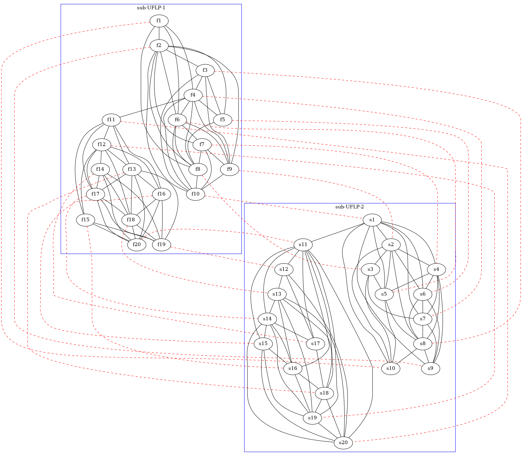
from jUFLP_utils import load_inst, draw_jUFLP_inst

i1, i2, link = load_inst("./instances/jUFLP_cm/inst_1.json")

draw_jUFLP_inst(i1, i2, link, filename="tmp/jUFLP-check.dot")

After this, variables i1, i2, and link will contain the j-UFLP instance description (respectively, the two sub-instances and the linking dictionary). Moreover, function jUFLP_utils.draw_jUFLP_inst() will create a .dot (Graphviz) file visualizing the instance as a graph, similar to Figure 9a. So that invoking dot -Tx11 tmp/jUFLP-check.dot (on my GNU/Linux machine) gives something like:

Code organization

The code is organized into several blocks (modules) as follows.

Producing figures

The code that physically produces figures from CSV run logs is written in R (and the wonderful tidyverse/ggplot2 library). The code is conceptually simple and, hopefully, self-explanatory – see .R - files in 📁 post_processing.

Key data structures and algorithms.

The core data structures critical to the paper are presented in the following modules (click on the links for more implementation details and the source code):

BDD	Implements the Binary Decision Diagram data type.
varseq	Implements weighted variable sequences data structure.
heuristics	Implements several heuristics to be used with a separate script to generate .csv logs.
BB_search	A branch-and-bound search scheme implementation for the align-sequences problem: alignts two varseq.VarSeq objects.

The code relevant to j-UFLP application (Section 4.2) is here:

UFL	Implements basic functions for UFL -- Uncapacitated Facility Location.
UFLP_fullDD	Solves UFLP using a DD-based approach.
UFLPOrder	Implements an algorithm to find a var order for BDD representing an UFLP.
jUFLP_cavemen	Proof-of-concept experiment: joint UFLP over special class of instances.
jUFLP_utils	Utility / helper functions for j-UFLP: used save / load / draw instances.

Numerical experiments

Description for specific problems serves the basis for further numerical experiments, which are implemented as separate python programs in 📁 experiments

gen_BDD_pair	Generates a pair of random BDDs ("original problem" instance).
solve_inst	Solves given align-BDD instances to benchmark different methods.
experiments	Implements most of the numerical experiments in the paper.
UFLP_2_cav	Generates and solves the special class j-UFLP instances.
darkcloud	Contains the j-UFLP instance generation code (along with some legacy experiments).

Testing framework

Key implementations are covered with tests, mostly using pytest framework. On top of the testing code in the files mentioned above (testing functions have test_ prefix in the name), some tests are in 📁 tests:

BDD_test	Tests some key procedures for BDD .
BDD_equivalence	Tests equivalence of BDDs after operations.
varseq_test	Tests the varseq.VarSeq procedures.
BB_search_test	Tests BB search correctness (BB_search)
UFLP_test	Tests the UFLP-related machinery (UFLP_2_cav and UFL).