On visualizing network graphs and Julia
Summary: Sometimes using specialized tools proves to be very convenient. To quickly visualize network graphs, I tried to use Graphviz program (invoking a stand-alone app from within Julia). It worked pretty well, both in terms of “UI” and the figures’ quality. Here I provide the minimal code I used and a couple complications, such as plugging in TeX with its PGF/TikZ instead of Graphviz (see also buttons below the title for source code files).
Of course, the idea is not new — see, e.g., PGFPlots.jl for a full-blown interface to PGFPlots — but hopefully demonstrates the point.
Discussion: I’d appreciate any comments / suggestions! Pls reach out via email.
Use-case and the problem
I have been working with networks in Julia and needed to quickly examine them visually. In particular, my use-case is that I am developing a graph-based algorithm and need:
- to look at an example instance graph. Usually, it is relatively small, up to several dozens of nodes.
- to visualize certain graphs decorated with additional data, such as a branch-and-bound search tree or Monte-Carlo search tree.
The package I am working with, LightGraphs.jl, does provide different ways to plot graphs by integrating with other packages, and this, of course, is a good starting point. However, for my specific (REPL-based) setup1 it just did not work nicely out of the box. Also, it perhaps required learning another domain-specific language (within Julia) for customizations. For example, I am doing Interdiction, and I want source and destination nodes filled with different colors. I might want even more freedom in formatting of a branch-and-bound tree. This is not bad per se, but I want to be sure that this new language is pretty good before learning it.
But then I thought, if I use R with (totally amazing) ggplot2 to visualize the data from csv files generated elsewhere — why not to do the same with graphs? Unix way and all… Apparently, this is both very easy to do and capable of producing nice output.
A quick, but efficient hack
My tool of choice for visualizing graphs from the previous project was a stand-alone program2 called Graphviz (dot command). To use it, I would just need to form and compile a plain-text .dot file written in DOT language. This is straightforward to do automatically. Assuming I have a SimpleDiGraph named G that I’d like to visualize, I can do:
open("./graph.tmp.dot", "w") do file
    write(file, "digraph {\n")

    for n in vertices(G)  # add nodes
        write(file,
              "    $n;\n")
    end

    for e in edges(G)  # add edges
        i=src(e); j=dst(e)
        write(file,
              "    $i -> $j;\n")
    end

    write(file, "}")
end
[What does this code produce?]
A resulting .dot file might look like this, for a five-nodes graph:
digraph {
    1;
    2;
    3;
    4;
    5;
    1 -> 2;
    1 -> 3;
    1 -> 4;
    1 -> 5;
    2 -> 3;
    2 -> 4;
    3 -> 4;
}
Now, this totally works, but I would need to compile it manually, that’s not user-friendly. Luckily, this is trivial to fix by adding:
run(pipeline(`dot -Tpdf ./graph.tmp.dot`,
             stdout="./graph.tmp.pdf"))
run(`xdg-open $filename.pdf`, wait=false)
(Note that these are backticks, `, not quotes '!)
So, it will produce ./graph.tmp.dot, compile it with the program dot, and open3 the resulting PDF with the default viewer in a separate window! (The REPL will not be blocked since we asked it not to with this wait = false.)
But wait, there’s more. It immediately gives us all the power of DOT language directly (which was, ehm, designed specifically to draw graphs!). Say, if I want to mark source and dest nodes with different colors, and show arc costs as well, I can modify the code above as follows:
"""Shows the graph with source node `s`,
dest `t`, and arc costs `W`."""
function showgraph(G, s, t, W,
                   filename="./graph.dot",
                   display=true)

    open(filename, "w") do file
        write(file, "digraph {\n")
        for n in vertices(G)  # add nodes
            if n == s
                style = "[style=filled, fillcolor=red]"
            elseif n==t
                style = "[style=filled, fillcolor=green]"
            else
                style = ""
            end
            write(file,
                  "    $n $style;\n")
        end

        for e in edges(G)  # add edges
            i=src(e); j=dst(e); cost=W[(i,j)]
            write(file,
                  "    $i -> $j" *
                      " [label=$(cost)];\n")
        end
        write(file, "}")
    end

    run(pipeline(`dot -Tpng $filename`,
                 stdout="$filename.png"))
    if display
        run(`xdg-open $filename.png`,
            wait=false)
    end
end
So, if I want to quickly look at graph G with source s, terminal t, and costs W, I just do showgraph(G,s,t,W) and a new window pops up:
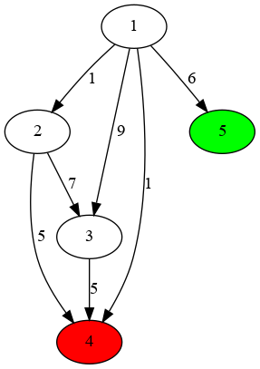
Now, if I want to examine two graphs (and save them as different files), I can call showgraph(G,s,t,W, "file1") and showgraph(G2,s2,t2,W2, "file2"). If I just want to update the file, without opening another window (e.g., if it is already open), I can ask to showgraph(G,s,t,W, "file", false).
Further improvement
Since we have just hacked the function together ourselves, it is really easy to modify. Assume I am drawing some more complicated things, and want to show more details about my nodes, which I have in names and info (indexed by the node number). Maybe, also format edge labels in some special way. It does not require any new ideas:
function showgraph_more(G, s, t, W,
                   names,
                   info,
                   filename="./graph.dot",
                   display=true)

    open(filename, "w") do file
        write(file, "digraph {\n")
        for n in vertices(G)  # add nodes
            if n == s
                style = "style=filled, fillcolor=red,"
            elseif n==t
                style = "style=filled, fillcolor=green,"
            else
                style = ""
            end

            label = "<<B>Name:</B> $(names[n])<BR/>" *
                "<B>Info:</B> $(info[n])<BR/>" *
                "<B>Node number:</B> $n>"

            write(file,
                  "    $n[$style label=$label]\n")
        end

        for e in edges(G)  # add edges
            i=src(e); j=dst(e); cost=W[(i,j)]
            write(file,
                  "    $i -> $j" *
                      " [label=\"added cost $(cost)\"];\n")
        end
        write(file, "}")
    end

    run(pipeline(`dot -Tpng $filename`,
                 stdout="$filename.png"))
    if display
        run(`xdg-open $filename.png`, wait=false)
    end
end
So, showgraph_more(G, s, t, W, names, info) again gives a picture in a new window:

(Here I used DOT markup: <B>...</B> for Bold, <SUB>...</SUB> for subscripts, and so on).
No doubt, DOT language is still somewhat limited, but again, it is a stand-alone, easy-to-plug tool. Also, we don’t discuss super-fancy publication-ready figures. Unless you want to…
Go TikZ!
Well, at this point nothing prevents us from employing even more complex tools, should we need some formatting heavy-lifting. There is basically no difference for us which “backend” to choose, even TeX-based! So, rewriting the simpler version of the function above for PGF/TikZ:
"""Draws a graph using TikZ."""
function showgraph_tikz(G, s, t, W,
                   filename="./graph",
                   display=true)

    # Let's insert some boilerplate styling
    # and necessary preamble/postamble
    preamble = """\\documentclass{standalone}
\\usepackage{tikz}
\\usetikzlibrary{graphs,graphdrawing,quotes}
\\usegdlibrary{force}

\\begin{document}
\\begin{tikzpicture}
  \\graph [spring layout, node distance=20mm,
 nodes={draw, circle, fill=blue, text=white},
  edge quotes={fill=yellow, inner sep=2pt}]
  {\n"""

    postamble = """};
\\end{tikzpicture}
\\end{document}"""

    open(filename * ".tex", "w") do file
        write(file, preamble)
        for n in vertices(G)
            if n == s
                style = "fill=red, text=white"
            elseif n==t
                style = "fill=green, text=black"
            else
                style = "fill=white, text=black"
            end

            write(file,
                  "    $n [as={\$n_{$n}\$}, $(style)];\n")
        end

        for e in edges(G)
            i = src(e); j = dst(e)
            cost = W[(i, j)]
            write(file,
                  "    $i ->[\"$(cost)\"] $j;")
        end
        write(file, postamble)
    end

    run(pipeline(`lualatex $filename`))
    if display
        run(`xdg-open $filename.pdf`, wait=false)
    end
end
[What does this code produce?]
That’s just a good old .tex file:
\documentclass{standalone}
\usepackage{tikz}
\usetikzlibrary{graphs,graphdrawing,quotes}
\usegdlibrary{force}

\begin{document}
\begin{tikzpicture}
  \graph [spring layout, node distance=20mm, nodes={draw, circle, fill=blue, text=white},
  edge quotes={fill=yellow, inner sep=2pt}]
  {
    1 [as={$n_{1}$}, fill=green, text=black];
    2 [as={$n_{2}$}, fill=white, text=black];
    3 [as={$n_{3}$}, fill=white, text=black];
    4 [as={$n_{4}$}, fill=red, text=white];
    5 [as={$n_{5}$}, fill=white, text=black];
    1 ->["1"] 2;    1 ->["9"] 3;    1 ->["1"] 4;    1 ->["6"] 5;    2 ->["7"] 3;    2 ->["5"] 4;    3 ->["5"] 4;};
\end{tikzpicture}
\end{document}
A call to showgraph_tikz(G,s,t,W) summons the unlimited power of TeX, so we spend some time looking at lualatex compilation log, but then indeed see a formatted digraph, as a PDF in a new window:
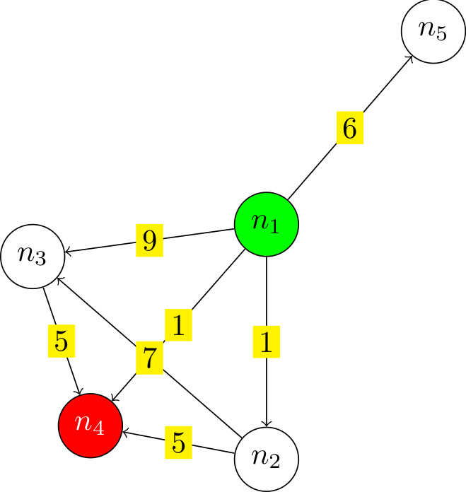
Of course, here we have all the tools (that was a link to a manual of more than 1,000 pages) of TikZ/PGF. We just generate and then compile a .tex file under the hood, nothing fancy.
In conclusion
So, while using TikZ seems like a little overkill for daily use, I really like the balance of simplicity and results with Graphviz. However, I might consider the former for producing the final versions of some figures and publication-ready supplemental materials next time.
Finally, while it seems really efficient as a quick and flexible tool, note that there are more general and, perhaps, tidy solutions that interface Julia and other systems — see, e.g., JuliaTeX with its PGFPlots, TikzGraphs / TikzPictures, and such. But hopefully this note illustrates the fact that sometimes using tools from seemingly different ecosystems might be pretty handy and simple.
Please, feel free to drop me an email if you’ll have any comments or suggestions!
-
My setup comprises my editor, Emacs, and Julia REPL running in a terminal side by side, with a decent degree of interactivity provided by Revise.jl. Many problems might be nonexistent, say, in Jupyter or VSCode. But that’s not the way I was ready to pursue at the moment, since I find the whole setting pretty convenient. ↩︎
-
Which I installed with
sudo apt install graphvizon my Debian system. (Would work the same way on Ubuntu, but you’d need tobrew install graphvizon Mac. There are options.) ↩︎ -
Technically speaking, this code will run on most Linuxes only, since I am using the program
xdg-open, which opens stuff in the default app. As far as I know, the Mac equivalent isopen. ↩︎